census.vars <- load_variables(2010, "acs5")Census Data
Features of Census data to note
The most popular surveys are the 1-Year and 5-Year American Community Survey (ACS), and the Decennial Census. This project mainly utilizes ACS5, which is available at the Census tract level from 2009 onward through the Census API. Earlier surveys (ACS1 starting from 2005) are only publicly available for geographies with larger population, typically the county level.
Census redraws boundaries every decade to reflect changes in population, thus Census tracts are delineated differently every 10 years and the data from different decades has to be “crosswalked”. This page provides code needed to query and crosswalk Census data. For details of geo-crosswalk, also see guidelines by NHGIS. NHGIS provides the geo-crosswalk files for mapping data from 2000s and 2020s to the 2010s vintage, which will be the baseline delineation of this project.
In light of the need for geo-crosswalk, only count data variables should be queried. For example, per capita income
B19301_001is the same as dividing aggregate incomeB19313_001by total populationB01003_001, but the former cannot be crosswalked, so as any ratio or percentage variables. For these variables, the corresponding numerators and denominators should be queried, crosswalked when needed, then divided to recover the desired ratio data. By the same token, median data variables should also be avoided.
1 tidycensus API
Census data can be queried directly in R using the package tidycensus (see its documentation). To see the complete list of variables that can be queried through the Census API, use load_variables,
Some variables that could be of interest to demographic and economic research are:
Note that ratio variables such as “per capita income” B19301_001 are shown for demonstration only and will not be used. The population of a block group/tract B01003_001 (almost the same variable as B03001_001) enables the calculation of crime rates and per capita data, such as dividing “Aggregate income” B19313_001 by it. However, it is important to note that when calculating averages, typically there is a specific denominator for a given “concept” and is not necessarily the total population. For example, to get average rent, one should divide “Aggregate gross rent” B25065_001 by “Total” B25063_001 which is the total number of renters, and the appropriate denominator for the concept “Gross Rent”, despite the label sounding otherwise.
The function get_acs can be used to query the ACS5 variables,
SF20 <- get_acs(geography = "tract", variables = "B01003_001", state = "CA",
                county = "San Francisco", year = 2020, geometry = TRUE)
The function can be wrapped inside a map_dfr (or the parallel version future_map_dfr) to get multiple variables from multiple years in one go,
get.census <- function(state.county, geography, years, variables, geometry = FALSE,
                       survey = "acs5", acs = TRUE, years.id = "year"){
  variables <- unname(variables)
  if (acs){
    temp <- future_map_dfr(
      years,
      ~ get_acs(
        geography = geography,
        variables = variables,
        state = state.county[[1]],
        county = state.county[[2]],
        year = .x,
        survey = "acs5",
        geometry = geometry,
        cache_table = TRUE
      ),
      .id = eval(years.id) # add id var (name of list item) when combining
    ) %>%
      arrange(variable, GEOID) %>%
      mutate(year = as.numeric(year) + min(years)-1)
  } else { # 2000, 2010, or 2020 only
    temp <- get_decennial(
      geography = geography,
      variables = variables,
      state = state.county[[1]],
      county = state.county[[2]],
      year = years,
      geometry = geometry
    )
  }
  return(temp)
}
Which can further be wrapped inside a lapply to loop through a list of state and counties, the multisession can also be planned here; the function returns a cleaned data in wide format,
get.census.list <- function(s.c.list, geography, years, variables, geometry = FALSE){
variables <- unname(variables)
plan(multisession, workers = parallelly::availableCores())
tic()
data.list <- lapply(s.c.list, function(x){
print(x)
temp <- get.census(x, geography, years, variables, geometry = geometry) %>%
select(year, GEOID, variable, estimate)
temp <- dcast(setDT(temp), year+GEOID~variable, value.var = "estimate")
})
toc()
return(rbindlist(data.list))
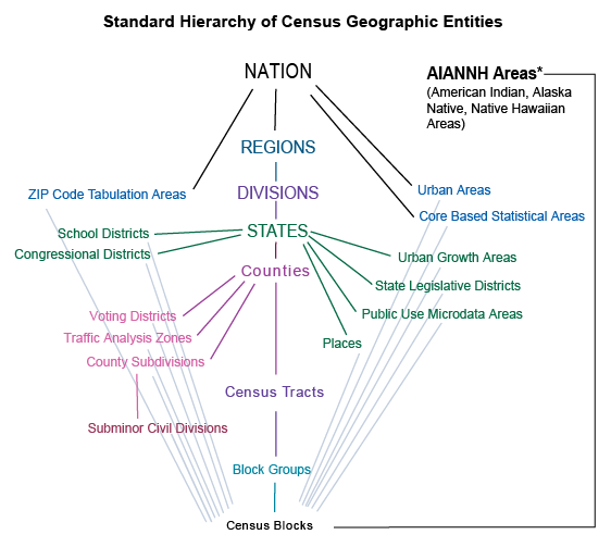
}2 Geographic crosswalk
As instructed by NHGIS, any variables to be crosswalked should start from the most granular, lowest possible level, meaning if a variable is available at the block (group) level, it should be used instead of the tract level to maximize accuracy.
Important: Start from the Lowest Level You Can To transform summary data from one census’s geographic units to another’s, it’s important to start from the lowest possible level.
This section provides a fully worked demo of querying and crosswalking 2020 block group count variables to 2010 tract, together with all the necessary code. In simplest terms, geo-crosswalk is achieved by calculating a weighted average that proportionately accounts for variation in geographical units. The variation could arise from redrawing of boundaries (e.g., 2010 Census tracts vs 2020 Census tracts) or from crossing levels (e.g., 2010 block groups vs 2010 counties); for example, a 10 year panel from 2015 to 2025 would span two vintages of Census boundaries, hence ACS5 estimates from 2015-2019 and estimates from 2020-2025 would originate from different neighborhoods. Geo-crosswalk harmonizes data into one single fixed geographical unit of analysis.
Census tract level population in San Francisco comparison
Suppose a project requires all analysis to be done at the 2010 tract level, and two variables available at the block group level from New York City and Chicago have to be queried and crosswalked when necessary (no crosswalk needed for the 2010-2019 estimates). The variables can be obtained using get.census.list shown above (note the nested structure of the state.county list); suppose only data from 2018 to 2021 are needed, the earlier two years can be queried at the tract level directly, while the later two should be queried at the block group level (lowest level available) then crosswalked,
# get population and aggregate income
vars <- c("B01003_001", "B19313_001")
# construct list of state-counties
state.county <- list(list("NY", list("New York", "Queens", "Kings", "Bronx", "Richmond")),
                     list("IL", list("Cook", "DuPage")))

# query variables separately, with intention to crosswalk
data.10s <- get.census.list(state.county, "tract", 2018:2019, vars)
data.20s.bg <- get.census.list(state.county, "block group", 2020:2021, vars)
With the 2020s data in block group, a “2020 Block Groups → 2010 Census Tracts” crosswalk file from NHGIS should be used. The crosswalk file contains these essential elements:
bg2020ge: GEOIDs of 2020 block groups, these are the “source” or “starting” geographiestr2010ge: GEOIDs of 2010 census tracts, these are the “target” or “ending” geographiesInterpolation weights, these are the weights to calculate the “weighted average”; the crosswalk file offers multiple weights, two of them are:
wt_pop: expected proportion of source geographies’ population in target geographieswt_fam: expected proportion of source geographies’ families in target geographies
and so on. Choice of weights depends on the nature of the variables and hopefully the weight chosen can reflect the spatial distribution of the variables of interest.
| bg2020gj | bg2020ge | tr2010gj | tr2010ge | wt_pop | wt_adult | wt_fam | wt_hh | wt_hu |
|---|---|---|---|---|---|---|---|---|
| G06003704017051 | 060374017051 | G0600370401701 | 06037401701 | 1 | 1 | 1 | 1 | 1 |
| G08003500146032 | 080350146032 | G0800350014603 | 08035014603 | 1 | 1 | 1 | 1 | 1 |
| G26012501444004 | 261251444004 | G2601250144400 | 26125144400 | 1 | 1 | 1 | 1 | 1 |
| G49001101255022 | 490111255022 | G4900110125502 | 49011125502 | 1 | 1 | 1 | 1 | 1 |
| G17015709506002 | 171579506002 | G1701570950600 | 17157950600 | 1 | 1 | 1 | 1 | 1 |
| G36011900131042 | 361190131042 | G3601190013104 | 36119013104 | 1 | 1 | 1 | 1 | 1 |
| G01012500127002 | 011250127002 | G0101250012700 | 01125012700 | 1 | 1 | 1 | 1 | 1 |
| G06008505093034 | 060855093034 | G0600850509303 | 06085509303 | 1 | 1 | 1 | 1 | 1 |
| G36000100003012 | 360010003012 | G3600010000300 | 36001000300 | 1 | 1 | 1 | 1 | 1 |
| G23001900090004 | 230190090004 | G2300190009000 | 23019009000 | 1 | 1 | 1 | 1 | 1 |
Leading zeros
When reading crosswalk files, be sure to keep leading zeros of GEOIDs (which are really character strings, not integers). For fread, you may use
formals(fread)$keepLeadingZeros <- getOption("datatable.keepLeadingZeros", TRUE)where the formals function changes the default values of fread and you might want to reset the value back to FALSE after reading GEOIDs.
The function that carries out the weighted average calculation is provided in full below, and it takes the following arguments:
crosswalk.file: a standard crosswalk file with source GEOID, target GEOID and interpolation weightscol.start: column name of the source column in the crosswalk filecol.end: column name of the target column in the crosswalk filecol.weight: column name of the interpolation weight columndata.walk: data that needs to be crosswalked (such as thedata.20s.bgqueried above)cols.walk: a single or vector of column/variable names that need to be crosswalkedcol.year: column name of the year column, in casedata.walkis in long format and contains multiple years
census.crosswalk <- function(crosswalk.file, col.start, col.end, col.weight,
                             data.walk, cols.walk, col.year = NULL){
  crosswalk.file <- as.data.table(crosswalk.file)
  data.walk <- as.data.table(data.walk)
  cols.walk <- unname(cols.walk) # just in case a named vector is passed

  # check data integrity
  if (any(!cols.walk %in% names(data.walk))){stop("Missing crosswalk columns!")}
  if (!("GEOID" %in% colnames(data.walk))){stop("GEOID not found in data.walk")}
  if (!all(unique(data.walk$GEOID) %in% crosswalk.file[, get(col.start)])){
    stop("GEOID does not exist in crosswalk.file, check if crosswalk file is correct")}
  if (!any(unique(data.walk$GEOID) %in% crosswalk.file[, get(col.end)])){
    cat("Note: Zero GEOID in col.end (expected for crosswalks across levels) \n")}
  if (!is.null(col.year)){
    years.mod = sort(unique(data.walk[, get(col.year)])) %% 10
    if (!all(sort(years.mod) == years.mod)){cat("Warning: Years not from same decade \n")}
  }


  # get desired group_by keys; year could be NULL
  cols.group <- c(eval(col.year), eval(col.end))

  temp <- crosswalk.file %>%
    # filter only relevant GEOID
    filter(!!rlang::sym(col.start) %in% data.walk$GEOID) %>%
    # select starting GEOID, ending GEOID, and weight columns
    dplyr::select(!!rlang::sym(col.start), !!rlang::sym(col.end), !!rlang::sym(col.weight)) %>%
    # right join data.walk and look up estimates of corresponding col.start
    right_join(data.walk, by = join_by(!!rlang::sym(col.start) == GEOID),
               keep = TRUE, relationship = "many-to-many") %>%
    # mutate/crosswalked variables; basically calculating a weighted average
    mutate_at(cols.walk, ~.x * get(col.weight)) %>%
    # aggregate back to a single row per GEOID per year
    group_by(across(any_of(cols.group))) %>%
    dplyr::summarise_at(cols.walk, ~round(sum(.x, na.rm = TRUE))) %>%
    # rename GEOID column to "GEOID"
    rename_with(~ "GEOID", !!rlang::sym(col.end))

  return(temp)
}
the upper part of the function performs a couple of validity checks to ensure that the proper information is supplied; the line
# get desired group_by keys; year could be NULL
cols.group <- c(eval(col.year), eval(col.end))
identifies potential keys that are used in group_by, see group_by(across(any_of(cols.group))) below. The lower chunk of code performs a right_join of the crosswalk.file and data.walk, keeping all rows in data.walk (the “right” data table); the two data tables are joined by matching the source GEOID in the crosswalk file and the GEOID in data.walk as expected because these are exactly the GEOIDs that need to be “turned into” the target GEOIDs. In the join function, relationship is set to"many-to-many" precisely to match the source GEOIDs to all the target GEOIDs, as one source GEOID may have 0.5 weight on target GEOID 1, 0.3 weight on target GEOID 2, and 0.2 weight on target GEOID 3 and so on. The data at this step will appear as follows:
# assuming validity checks are all passed
temp <- crosswalk.file %>%
  # filter only relevant GEOID
    filter(!!rlang::sym(col.start) %in% data.walk$GEOID) %>%
    # select starting GEOID, ending GEOID, and weight columns
    dplyr::select(!!rlang::sym(col.start), !!rlang::sym(col.end), !!rlang::sym(col.weight)) %>%
    # right join data.walk and look up estimates of corresponding col.start
    right_join(data.walk, by = join_by(!!rlang::sym(col.start) == GEOID),
               keep = TRUE, relationship = "many-to-many") %>%
    # mutate/crosswalked variables; basically calculating a weighted average
mutate_at(cols.walk, ~.x * get(col.weight))| bg2020ge | tr2010ge | wt_pop | year | GEOID | B01003_001 | B19313_001 |
|---|---|---|---|---|---|---|
| 170438418023 | 17043841403 | 0.0099870 | 2020 | 170438418023 | 14.6709490 | 650914.75 |
| 170438418023 | 17043841403 | 0.0099870 | 2021 | 170438418023 | 15.4199763 | 707614.12 |
| 170438418023 | 17043841802 | 0.9900130 | 2020 | 170438418023 | 1454.3290510 | 64525085.25 |
| 170438418023 | 17043841802 | 0.9900130 | 2021 | 170438418023 | 1528.5800237 | 70145685.88 |
| 170438419011 | 17043841901 | 0.9991683 | 2020 | 170438419011 | 1219.9844781 | 71993771.98 |
| 170438419011 | 17043841901 | 0.9991683 | 2021 | 170438419011 | 1343.8813456 | 82107553.21 |
| 170438419011 | 17043842000 | 0.0008317 | 2020 | 170438419011 | 1.0155219 | 59928.02 |
| 170438419011 | 17043842000 | 0.0008317 | 2021 | 170438419011 | 1.1186544 | 68346.79 |
| 170438419012 | 17043841901 | 1.0000000 | 2020 | 170438419012 | 1478.0000000 | 94718100.00 |
| 170438419012 | 17043841901 | 1.0000000 | 2021 | 170438419012 | 1509.0000000 | 109408500.00 |
| 170438419021 | 17043841902 | 0.9982555 | 2020 | 170438419021 | 1457.4529844 | 45351744.20 |
| 170438419021 | 17043841902 | 0.9982555 | 2021 | 170438419021 | 1437.4878751 | 50558544.90 |
| 170438419021 | 17043842200 | 0.0002732 | 2020 | 170438419021 | 0.3988285 | 12410.40 |
| 170438419021 | 17043842200 | 0.0002732 | 2021 | 170438419021 | 0.3933651 | 13835.22 |
| 170438419021 | 17043842300 | 0.0014714 | 2020 | 170438419021 | 2.1481869 | 66845.40 |
| 170438419021 | 17043842300 | 0.0014714 | 2021 | 170438419021 | 2.1187597 | 74519.87 |
| 170438419022 | 17043841902 | 1.0000000 | 2020 | 170438419022 | 2764.0000000 | 50470200.00 |
| 170438419022 | 17043841902 | 1.0000000 | 2021 | 170438419022 | 2765.0000000 | 51279100.00 |
| 170438420001 | 17043842000 | 0.9981638 | 2020 | 170438420001 | 1209.7745481 | 80541439.26 |
| 170438420001 | 17043842000 | 0.9981638 | 2021 | 170438420001 | 1096.9820366 | 88056115.57 |
# mutate/crosswalked variables; basically calculating a weighted average
mutate_at(cols.walk, ~.x * get(col.weight))
this line mutate all columns that are passed to cols.walk by multiplying with the interpolation weight column (wt_pop here); this is basically the first part of a vector multiplication/weighted average calculation, and the subsequent group_by and summarise with sum take care of the “summation” part of the calculation. The resulting data set would represent 2020 and 2021 population (B01003_001) and aggregate income (B19313_001) but in 2010s Census tract.
| year | GEOID | B01003_001 | B19313_001 |
|---|---|---|---|
| 2020 | 17031010100 | 4644 | 185453100 |
| 2020 | 17031010201 | 7488 | 172679400 |
| 2020 | 17031010202 | 3154 | 70535900 |
| 2020 | 17031010300 | 6135 | 212985000 |
| 2020 | 17031010400 | 5193 | 124331800 |
| 2020 | 17031010501 | 4039 | 128187900 |
| 2020 | 17031010502 | 2960 | 80647000 |
| 2020 | 17031010503 | 1973 | 38529700 |
| 2020 | 17031010600 | 6363 | 247171600 |
| 2020 | 17031010701 | 3562 | 111193500 |
| 2020 | 17031010702 | 5209 | 117978100 |
| 2020 | 17031020100 | 3742 | 123427200 |
| 2020 | 17031020200 | 6980 | 259245900 |
| 2020 | 17031020301 | 5447 | 163901700 |
| 2020 | 17031020302 | 5116 | 222301500 |
| 2020 | 17031020400 | 4011 | 170245300 |
| 2020 | 17031020500 | 6744 | 115295500 |
| 2020 | 17031020601 | 6112 | 172181800 |
| 2020 | 17031020602 | 5239 | 151466200 |
| 2020 | 17031020701 | 1764 | 76773200 |
Using the same code, crosswalks from 2000s vintage, across different levels of nested geographies, with data from multiple states/counties or variables can easily be done by changing only the relevant items, such as supplying the appropriate crosswalk file.
Do NOT crosswalk ratio or median variables
Again, the idea of crosswalking is to distribute a variable based on interpolation weights from one geography to another, thus it does not make sense to crosswalk variables that are not some sort of counts. You can test this by trying to crosswalk “per capita income” B19301_001, and you will see that the results are unreasonable. Clearly the same idea applies to median variables.
3 Variable operations
Once the data is queried (and stored in an object called census.data), any desired ratio variables or other transformations can be obtained or carried out; variables can also be given some easy-to-understand common.name. To avoid coding mistake/oversight and to streamline the workflow, it is strongly advised that the calculations be done dynamically (i.e., not hard coding the operations and not writing one line of code for each calculation). Taking the queried Census data from above, the code below will finish the task dynamically; although it is inevitable that for each ratio to be calculated, the numerator and denominator needs to be recorded somewhere, the procedure should minimize the chance of error.
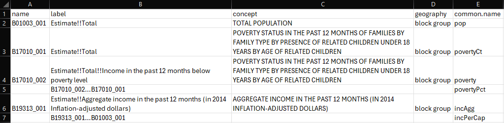
Suppose the variables taken from
load_variablesare stored in a.csvfile, a new columncommon.namecan be created to store user-defined names that will replace the Census variablenamein a later step.For each new variable to be created, store the numerator and denominator needed in the column
label(or any other columns deemed fit), leaving thenamecolumn empty. The format should be [numerator][separator][denominator], where...is used here (because ÷ looks like three dots). To accommodate other operations including ones involving more than 2 variables, you can use a distinct operator for each type of operation and adapt the code accordingly. Also note how each ratio is defined very close to its “ingredients” to prevent mistakes when copy-pasting.
- Create new variables by looping through any rows with a
common.namebut without aname. The code can be parallelized but given this is a small scale column-wise operation, it is unlikely that there will be significant performance gain.
# include this line if you have not already set proper na.strings
formals(fread)$na.strings <- c("", "NA", "N/A", "(null)", "NULL", "null")

census.vars <- fread("census.variables.csv")

for (x in census.vars[is.na(census.vars$name),]$common.name){
  row <- census.vars[census.vars$common.name == x, ]

  # variables separated by ... are to be divided
  # load the "zeallot" package to use the %<-% operator
  c(numer, denom) %<-% strsplit(row$label, split = "\\.\\.\\.")[[1]]
  census.data <- census.data %>%
    mutate(!!rlang::sym(x) := get(numer) / get(denom))
}

# clean up NaN's produced by zero dividing by zero
census.data <- census.data %>% mutate_all(~ifelse(is.nan(.), NA, .))
na.strings
When reading the csv file, to ensure that an empty cell will be interpreted as NA, make sure to set the na.strings (or equivalent) of your reading function to include "". You can also read file or files by using pattern of the file names and search recursively under the working directory using list.files with recursive = TRUE.
- Set original variables to
common.names. The following code assumes that for all variables, there is acommon.name, so any variables with non-NAnamecan be matched with one. If this is not the case, simply loop through variables that need to be renamed instead.
census.data <- census.data %>%
  setnames(census.vars[!is.na(census.vars$name),]$name,
           census.vars[!is.na(census.vars$name),]$common.name)
Step 3. and 4. can be interchanged, but doing so will add a layer of dependency as the label column needs to be updated every time a common.name is changed, while name is basically not going to change.
Copyright © April 2025. Hung Kit Chiu.