Geocoding

Data with street addresses but not coordinates can still be mapped to Census tracts with geocoding - converting address to coordinates. To fully leverage publicly available data, this project uses a combination of two geocoding services to carefully geocode incidents. This document provides a detailed description of the workflow of incorporating geocoding into a bigger project, especially doing so in a completely open source manner without sacrificing quality.

Esri ArcGIS Pro

Esri is a leading provider of GIS (Geographic Information System) technology. Its product, ArcGIS Pro, offers bulk geocoding tools such as “Geocode Addresses” in the geocoding toolbox. Users who are subscribed to ArcGIS services can batch geocode addresses directly from within ArcGIS Pro. Refer to the documentation for details.

Nominatim/OSM

Nominatim is a free, open-source geocoding service based on OpenStreetMap (OSM). It is capable of forward geocoding (converting addresses into geographic coordinates) and reverse geocoding (coordinates to addresses). While it is possible to use the public Nominatim API provided by OSM, users are limited to one query per second. This project hosts its own instance due to heavy usage. The Nominatim website offers clear and actively maintained documentation, including step-by-step installation guides for running it on various Linux systems.

This section is fully opensource, based on Ubuntu 24.04 LTS, PostgreSQL 17.5, Nominatim 5.1.0, Python 3.12 and the North America extract north-america-latest.osm.pbf from Geofabrik in May 2025. Needless to say, this project also uses R, RStudio and Quarto; I thank all open-source contributors.

Installation

For a basic installation of Nominatim, follow the official installation manual using the latest Linux distribution. You will need:

• PostgreSQL with PostGIS

• PHP, Python, and supporting libraries

• Nominatim source code (via GitHub or package manager)

• Adequate system resources (e.g., 64 GB RAM for continent-scale imports)

The installation manual also covers software dependencies, PostgreSQL tuning, and how to import OSM .pbf data into your local Nominatim database. The manual also includes links to various containers/dockers that might suit your needs.

A full import of May, 2025 version of north-america-latest.osm.pbf will use about 300GB of disk space and more than 24 hours for consumer level computers. The import was tested on a machine with Intel Core i5-9400 6-Core Processor, 64 GB RAM and 1 TB Gen 3 NVMe SSD.

The basic installation enables geocoding of addresses involving only a single location, however, to geocode addresses in the form of intersections and to fully reproduce the results presented on this page, additional imports of the osm_raw database is needed; the import uses the same north-america-latest.osm.pbf file and adds more information on top of the Nominatim database. Most notably the planet_osm_line and planet_osm_polygon tables will be used to figure out intersections of streets or polygons such as parks via a robust fallback sequence to be discussed in Section 2.3. The osm_raw database will contain tables such as:

• planet_osm_line: roads, rail, footpaths, etc.

• planet_osm_point: point of interests (POIs)

• planet_osm_polygon: buildings, land use

This import took about 7 hours on a decently configured machine and used roughly another 300GB of disk space. Also, be sure to index the name columns of both the planet_osm_line and planet_osm_polygon tables.

CREATE INDEX planet_osm_line_name_idx ON planet_osm_line (name); 
CREATE INDEX planet_osm_polygon_name_idx ON planet_osm_polygon (name);

Finally, to allow for fuzzy name matching - in case there is no match for a street, look for similarly named alternatives using Levenshtein distance and similarity, follow these steps in the terminal,

1. Going into the osm_raw database,

sudo -u postgres psql -d osm_raw

You should see the osm_raw# prompt waiting for SQL inputs.

2. Create the extensions unaccent, pg_trgm, and fuzzystrmatch,

CREATE EXTENSION IF NOT EXISTS unaccent;
CREATE EXTENSION IF NOT EXISTS pg_trgm;
CREATE EXTENSION IF NOT EXISTS fuzzystrmatch;

3. Create GIN indexes for the planet_osm_line and planet_osm_polygon tables on the column name so that the fuzzy lookups can filter the candidates using similarity before calculating Levenshtein distance; note that this step will take some time to run, do not disturb the process.

CREATE INDEX IF NOT EXISTS idx_line_name_trgm_gin ON planet_osm_line USING gin (lower(name) gin_trgm_ops);
CREATE INDEX IF NOT EXISTS idx_polygon_name_trgm_gin ON planet_osm_polygon USING gin (lower(name) gin_trgm_ops);

alternatively, GiST indexes can also be created. For comparison between GiST and GIN, see the documentation of PostgreSQL.

CREATE INDEX IF NOT EXISTS idx_line_name_trgm_gist ON planet_osm_line USING gin (lower(name)gist_trgm_ops);
CREATE INDEX IF NOT EXISTS idx_polygon_name_trgm_gist ON planet_osm_polygon USING gin (lower(name) gist_trgm_ops);

Batch geocoding

Suppose an installation is complete and the database is set up properly (with virtual environments and permissions, etc. correctly configured), the following logic and code can be used to perform batch forward geocoding using a self-hosted Nominatim instance. Two sequential python scripts geocode.py and geocode_pass2.py are used. Assuming the inputs are well-formatted, the first pass should handle more than half of the addresses and will produce a list of unmatched addresses to be processed further. The second pass will run much slower with additional parsing of addresses and will handle addresses with tricky formats, such as i) intersections of two streets, ii) parallel streets, iii) close but non-intersecting streets, which are all common in crime data sets to preserve anonymity. Nominatim is not really designed to handle these addresses natively, despite being able to match each street individually. The script will query the raw OSM database to find coordinates of geographic intersections, potentially with a 500m proximity buffer to geocode streets that are close or parallel but do not intersect.

graph TD

  %% Core flow
  A1[address.csv] --> B1[geocode.py]
  B1 --> C1[geocoded_matches.csv]
  B1 --> C2[geocoded_unmatched.csv]
  C2 --> B2[geocode_pass2.py]
  B2 --> C3[geocoded_pass2_matches.csv]
  B2 --> C4[geocoded_pass2_unmatched.csv]

  %% Support files
  D1[name_cleanup_rules.csv] --> E1[geofunctions.py]
  E1 --> B1
  E1 --> B2
  F1[city_viewboxes.csv] --> B2

  %% Helper Tools
  subgraph hps [Helper scripts]
    H1[extractcol.py]
    H2[countsuffix.py]
  end

  C4 -.-> H1
  C4 -.-> H2
  H1 -.-> D1
  H2 -.-> D1
  
  style hps fill: lightgray

Figure 1: Batch geocoding workflow and dependency

Splitting the workflow into two separate scripts is deliberate and the first script is designed to be light and fast with minimal parsing and queries (the user is expected to feed it reasonably formatted addresses, see Tip 1 and Section 3.1). The match rate obviously depends on how well-formatted the addresses are and how detailed the coverage of OSM is in the area, in any case, the user should inspect what is not matched in geocoded_unmatched.csv to hopefully identify patterns of quirkiness that prevent matching and adapt the second script geocode_pass2.py accordingly. The second script is designed to carry out extra parsing of addresses using mapping provided by name_cleanup_rules.csv and handle intersections that frequently occur in crime data, all within a bounding area specified in city_viewboxes.csv. User can define custom mapping of abbreviations such as locally used aliases in name_cleanup_rules.csv. The workflow ends with iterating through multiple versions of edits by repeatedly checking what is left in geocoded_pass2_unmatched.

Input format

Start by preparing an address.csv file containing a single column named address, with each row being one address in the format of [street], [city], [state]. This file will go into the first geocoding script. If you are trying to geocode addresses that exist in a larger data set, you will want to use these inputs as keys that will help you join the geocoding results back to the original data set, which means i) the addresses are unique and ii) in the original data set, there is a column that contains the exact same addresses (which may have duplicates); no parsing should be done in between that column and the address.csv. Example of adress.csv,

address
"2100 Scott Blvd, San Jose, CA"
"123 Main St, San Francisco, CA"
"1 Infinite Loop, Cupertino, CA"
"Mission Blvd & Warm Springs Blvd, Fremont, CA"

Some checks (by no means comprehensive) for the addresses,

• they have no leading or trailing spaces, which will cause two otherwise identical addresses to be interpreted as distinct

• they are unique with keys set up properly in the original data set

• they end with two letter state abbreviation, with city immediately preceding state, separated by a comma

the third condition is required for the geocode_pass2.py to work properly as it will attempt to extract city using the code

def extract_city(address):
  parts = address.split(',')
  return parts[-2].strip().lower() if len(parts) >= 2 else None

Tip 1: Trying out addresses

To get a sense of how addresses should be formatted, you can always try searching them on OpenStreetMap.org, and if it returns a search result, most likely your addresses are ready.

geocode.py

This script performs an initial geocoding pass, it

• Sends each address to the nominatim/search endpoint.

• Saves results in two csv files:

  • geocoded_matches.csv - successful matches

  • geocoded_unmatched.csv - plain list of failed addresses

• Displays a real-time progress bar using tqdm.

• Reports percentage of failed matches at the end.

geocode_pass2.py

Using the osm_raw database, the second pass script geocode_pass2.py does the following:

• Standardize addresses using definitions in the two dictionaries ABBREVIATION_MAP and DIRECTION_MAP

• Tries single addresses after parsing again and returns the result

• Detects intersection-style addresses (e.g., "X St & Y St")

• Checks if both street exists individually in the data base, if yes,

  1. Queries the raw OSM database to find any geographic intersection of streets, if this fails,

  2. Queries the raw OSM database to find any false intersection of streets with BUFFER_DISTANCE = 500 (in meters), stopping as soon as a match is found.

• Outputs a matched file geocoded_pass2_matches.csv and an unmatched file geocoded_pass2_unmatched.csv

To obtain a more refined result and to limit the search space, the script will need to know the boundary to search, this information is passed on from a city_viewboxes.csv containing two columns with city name (that has to match exactly with the one used in addresses) and two pairs of latitude and longitude coordinates that trace out a viewbox (also called a “bounding box”), to use the viewbox file with the code below, obey the order of “left, top, right, bottom” or “minLon, maxLat, maxLon, minLat”, which correspond to the northwest and the southeast corners,

city,viewbox
San Jose,"-122.05,37.40,-121.75,37.20"
Fremont,"-122.10,37.60,-121.80,37.40"

Buffer size, false intersection, and viewbox

An actual intersection tested when building the code is CLOVBIS AV & BLOSSOM HILL RD, San Jose, CA, which do not intersect but appear pretty close on a map. This is known as a “false intersection”. The address might have been entered this way because the exact location of the incident was not identified; the script will approximate the closest point of the two streets based on a fuzzy match.

The code is restricting (not merely biasing) the search to within the viewbox for a given city, and within a buffer size for possible intersections; for two streets that do not intersect but are both found in the database, their centroid is taken as the geocoded location if their closest segments are within the buffer size. Obviously by this logic, a larger viewbox and buffer size will increase the likelihood of matching (and false positives), less obviously they also lead to longer code run-time. In fact, significantly longer if a viewbox is not used at all because the code will try to search through all intersections with name match in North America and return the first geographic match, which is why the code enforces viewbox and will not run if one is missing.

This treatment of viewbox is different the standard industry practice but necessary for a local instance to keep runtime under control. A commercial API typically uses viewbox as a biasing mechanism and will consider strong matches outside of a city to cater so as to a wider range of use cases. Imposing a strict boundary, however, is very practical for this project because the data comes from city-level law enforcement agencies, meaning it is certain that incidents will be within or near a city, thus using a somewhat “relaxed” viewbox (one that is slightly larger than the police department’s jurisdiction) will be ideal for efficiency while still having enough buffer to account for incidents that potentially happen outside of the city limits (such as in adjacent unincorporated areas or a bordering town for mutual aid).

Example output in geocoded_pass2_matches.csv:

original_address,used_variant,lat,lon,result
"250 COY DR, San Jose, CA","250 COY DR, San Jose, CA",37.255,-121.824,"Coy Drive, San Jose, Santa Clara County, California, 95123, United States"
"250 N MORRISON AV, San Jose, CA","250 N MORRISON AV, San Jose, CA",37.333,-121.908,"North Morrison Avenue, College Park, Buena Vista, San Jose, Santa Clara County, California, 95126, United States"
"2150 CORKTREE LN, San Jose, CA","2150 CORKTREE LN, San Jose, CA",37.417,-121.866,"2150, Corktree Lane, San Jose, Santa Clara County, California, 95132, United States"
"QUIMBY RD & S WHITE RD, San Jose, CA","QUIMBY RD & S WHITE RD, San Jose, CA",37.325,-121.797,"Quimby Road & South White Road, Quimby Road, San Jose, Santa Clara County, California, 95148, United States"

geofunctions.py

Helper functions that facilitate both geocode.py and geocode_pass2.py by parsing reference files and creating address variants to be used in the fallback sequence (Section 2.3) when the raw address does not return a match.

• expand_abbreviations(address) converts street suffix abbreviations to their full names as included in name_cleanup_rules.csv, which contains all abbreviations presented by USPS, plus many more. Note that the abbreviation “St” is handled separately and should not be included in name_cleanup_rules.csv, due to conflict caused by “Street” and “Saint”.

• expand_directions(address) converts direction abbreviations to their full names, such as N to North or SW to Southwest.

Helper scripts

• extractcol.py extracts the address column from a geocoded_pass2_unmatched.csv which contains 5 columns, the extracted addresses can then be geocoded again after potentially adding more naming rules to name_cleanup_rules.csv.

• countsuffix.py looks at un-coded addresses that appear the geocoded_pass2_unmatched.csv and finds high-frequency suffixes that are not already addressed in name_cleanup_rules.csv. This could help identify local aliases that are preventing a match.

These two scripts are used in Section 3.2 of the demo.

Fallback logic

The raw address coming from the source is the original_address and it is fairly common that these raw addresses return no-match despite the actual street “existing” in one way or another in the database due to sorts of complications associated with character string data and spatial data. To increase match rate without sacrificing accuracy, conditional on an address being unmatched, a sequence of fallbacks are constructed and retried until there is a match or until all variants are exhausted. The design and order of these fallbacks are informed by trials and errors with addresses from multiple US cities.

Figure 2 and Figure 3 show the fallback logic embedded in geocode_pass2.py; addresses are distinguished into single address type that goes on to query Nominatim and intersection type that goes on to query the PostGIS raw database. Every address will be queried in its original form first before moving onto the next variant, in the sense that geocode_pass2.py can work by itself without having to feed addresses to geocode.py first. All queries are made with the restriction of viewbox, and from variants that are closer to the original to less, and hence “fallback” figuratively.

flowchart LR
  A[1#46; original_address] --> B[2#46; abbr_expand]
  B --> D
  A --> C[3#46; dir_expand] --> D[4#46; full_expand]
  D --> E[5#46; remove_city] --> F[6#46; remove_suffix]
  D --> G[7#46; fuzzy_name]
  D --> H[8#46; fuzzy_suffix]

Figure 2: Address variants, tried sequentially, exiting on first match

For each address, each variant is tried sequentially until a match; for single address type, it tries Nominatim and the result will be hit or miss, for intersection type, there is an added layer of fallback, with works for intersections of line or polygon,

flowchart LR
  A[exact_intersection] --> B[buffer_intersection] --> C[average_centroid]

Figure 3: Sequence of fallbacks for intersections/PostGIS queries

Brief explanations regarding each variant,

1. Unaltered, verbatim address as appeared in data

2. Expanding abbreviations and suffixes that are covered in name_cleanup_rules.csv (excerpt shown below), except those with the “Fuzzy suffix” in the “notes” column (which will be used in variant 8). The “match” column can take both plain text and regular expressions and the “replace” column stores the corresponding replacement. The default of the replacement is done with word boundaries (\b), but including “no-boundary” in the “notes” column will trigger the code to not use boundaries. Any rows with the word “suffix” will trigger the function remove_suffix in variant 6. All replacement is done in a case-insensitive manner, so the strings can appear with any capitalization in both the source data, and in the name_cleanup_rules.csv.

match,replace,notes
BL,Boulevard,Common suffix
BLVD,Boulevard,Alternative abbreviation
C,Circle,Fuzzy suffix
C,Court,Fuzzy suffix
Martin Luther King JR,Martin Luther King Junior,Berkeley name

and although this variant is called “abbr_expand”, it really means replacement of any words, or even removal of words if that facilitates matching, for example, the following also works seamlessly,

NEW AUTUMN ST,N Autumn Street,San Jose name/typo
th Half st, 1/2 street,Virginia Beach name/no-boundary
st half st, 1/2 street,Virginia Beach name/no-boundary
nd half st, 1/2 street,Virginia Beach name/no-boundary
rd half st, 1/2 street,Virginia Beach name/no-boundary
Dead End,,San Jose
Mbta,,Cambridge

and if an intersection style address becomes a single street after word replacement, the intersection connector will be dropped, for example, the following actual address from San Jose gets turned into the corresponding variant and gets a match (albeit an imperfect one, because only the centroid of “Silver Ridge Drive” is returned as it is hard to determine which “Dead End” the data is referring to)

"DEAD END & SILVER RIDGE DR, San Jose, CA" → "SILVER RIDGE Drive, San Jose, CA"

And repeating what is said above, > Note that the abbreviation “St” is handled separately and should not be included in name_cleanup_rules.csv, due to conflict caused by “Street” and “Saint”.

3. Expanding the basic 8 direction abbreviations, “N” becomes “North”, “NE” becomes “Northeast” and so on.

4. Putting abbreviation expansion (or word replacement) and direction expansion together.

5. Removing city from the address, but the geocoding is still subject to the viewbox and thus an address will not be matched to a distant place. The variant is put in place to handle issues caused by an address being in a big city but not exactly in that city. For example, an actual address from the San Jose data is “2500 GRANT RD, San Jose, CA” which will fail the match because the address is actually in the city Mountain View, this step creates the variant “2500 GRAND RD, CA” and will get a match; another example is “1950 YELLOWSTONE AV, San Jose, CA” that only yields a match with the variant “1950 YELLOWSTONE AV, CA” as the address is actually in Milpitas. To reiterate, despite the city being removed, the search is still done within the viewbox (which is designed to be a bit larger than the city, consistent with how city police departments operate), so in the previous examples it does not mean the search is done in the entire state of California.

6. Removing suffix from the address, by suffix it means any rows with the keyword “suffix” in the “notes” column of name_cleanup_rule.csv. For example, the following is an actual match from San Jose, where “HELLYER Avenue & FONTANOSO Road” failed to yield a match because it is actually “Fontanoso Way” not “Fontanoso Road”, dropping suffix yields an accurate match,

"HELLYER AV & FONTANOSO RD, San Jose, CA","hellyer & fontanoso, ca",37.2634285,-121.7879597,PostGIS: Intersection hellyer & fontanoso

7. Searching for streets with very close names. See @note-fuzzy_name.

8. Trying multiple possible suffixes, this happens when an address comes with an ambiguous suffix such as “C” which could mean “Court” or “Circle” or “P” which could mean “Park” or “Place”, each possible suffix will be tried one by one in the order they appear in name_cleanup_rules.csv. *This step happens conditional on the address not getting a match in the remove suffix variant (technically the remove suffix step can be modified to not remove ambiguous suffixes, this practice is currently still subject to trial and errors).

Levenshtein distance and fuzzy name fallback

For all intents and purposes here, the Levenshtein distance between two strings is the minimum number of single-character edits (insertions, deletions, substitutions, etc.) required to change one string into the other. For example, the Levenshtein distance between “extensive” and “exhaustive” would be 3. A Levenshtein distance of 1 would account for common data artifacts such as missing spaces or (single) letters, or extra hyphens or periods, etc.

Strings often fail to match due to minor typos, this can be addressed using PostgreSQL’s fuzzystrmatch where closely named streets could be identified by calculating the Levenshtein distance on all candidate streets shortlisted by viewbox and similarity filtering. The function find_similar_street in geocode_pass2.py finds all streets, within the viewbox, that have a Levenshtein distance of 1 or lower from the target street, and return the most similar street except when that is the target street itself; by similar it means the highest similarity using PostgreSQL’s pg_trgm.

Using address from Saint Paul as an example, the code can successfully match these following addresses (compare the “original_address” and the “used_variant”),

original_address,used_variant,lat,lon,result
"2595 CROSBYFARM RD, Saint Paul, MN","2595 Crosby Farm Road, Saint Paul, MN",44.896,-93.169,Nominatim match
"1575 LORIENT ST, Saint Paul, MN","1575 L'Orient Street, Saint Paul, MN",44.988,-93.090,Nominatim match
"185 GENESEE ST, Saint Paul, MN","185 Genessee Street, Saint Paul, MN",44.965,-93.092,Nominatim match
"1585 EASTSHORE DR, Saint Paul, MN","1585 East Shore Drive, Saint Paul, MN",44.985,-93.048,Nominatim match

For even more details about the fallback logic, see functions process_address and try_postgis_intersection in the source code geocode_pass2.py, and potentially any helper functions called from geofunctions.py.

Demonstration

Both Esri ArcGIS Pro and Nominatim with OSM raw database were used to geocode street addresses in multiple US cities. Either approach achieves fairly high level of accuracy and offers room for tuning, but the self-hosted Nominatim instance certainly allows for more flexibility. This section showcases geocoding using Nominatim/OSM.

Preparation

Addresses should be parsed before compiling the address.csv of unique addresses. Here are some common treatments for addresses seen in crime data, assuming the target vector is named address,

1. De-censorship. gsub("(\\d+)X", "\\15", address, perl = TRUE) converts a number-followed-by-X pattern into a number.

"205X SUMMIT AVE, Saint Paul, MN"  →  "2055 SUMMIT AVE, Saint Paul, MN"

2. Intersection connectors. str_replace_all(address, some_separator, "&") converts any occurrences of some peculiar connector into & (the only intersection separators coded into the script are &, AND (case insensitive), and /, note also that AND could conflict with place names). Suppose + is such peculiar connector,

"EDWARDS AV + WILLOW ST, San Jose, CA"  →  "EDWARDS AV & WILLOW ST, San Jose, CA"

3. Word removal. str_remove_all(address, " BLOCK") removes the superfluous word  BLOCK

"2900 BLOCK S 72ND ST"  →  "2900 S 72ND ST"

4. Spacing. The following cleans up spaces in and around the address to ensure uniqueness.

# trim leading and trailing spaces
across(any_of(address.cols), trimws)
# remove any extra spaces
address.clean = gsub("\\s+", " ", address.clean, perl = TRUE)
# remove any one space before a comma
gsub("(?<=[A-Za-z0-9])\\s+,", " ", address.clean, perl = TRUE)

5. Adding suffix when needed. paste0(address, ", City, State") adds the city and state to a street address.

6. Other parsing. Any other city-specific parsing should be done prior to geocoding, take San Jose as an example,

"[2900]-[3000] ALMADEN RD"  →  "2950 ALMADEN RD, San Jose, CA"

7. Generating unique addresses. address <- unique(address) selects non-duplicated addresses.

Iteration

Once the addresses are prepared, the following process can be carried out and iterated until, theoretically, all addresses are matched. This is the biggest advantage over using a commercial API as artifacts in the source can be iteratively identified and addressed, and running the algorithm repeatedly does not add to the cost.

It should be noted that, from experience, many problematic addresses need to be intervened before being fed into commercial APIs, which has a tendency to brute force a match (i.e., they go by the philosophy of returning something is better than returning nothing), and artifacts will only lead to incorrect mapping that could go undetected. In contrast, with the framework presented here, problematic addresses will simply be unmatched and isolated, which can then be fixed, as the examples in Step 3 show.

1. Run geocode.py to quickly match addresses; the match rate of this step depends on the quality of the data.

2. Inspect gocoded_unmatched.csv to see if there are any aliases that prevent matching, or if there are other issues that should have been addressed in the Preparation step. This could involve going back and forth between the unmatched addresses and OpenStreetMap.

3. Update name_cleanup_rules.csv to incorporate more aliases to proper names conversion. The countsuffix.py script may be helpful, below presents some examples. Converting “MTIDA” to “MOUNT IDA” in Saint Paul is a more intricate one; the code can handle \bMt\b (“Mt” sandwiched between word boundaries) which will be expanded to “Mount”, and the code can handle streets that are mis-typed by missing one space, so “MT IDA” or “MOUNTIDA” would have worked without having to manually enter a mapping, but the code cannot handle complex issues.

match,replace,notes
M L King JR,Martin Luther King Junior,Berkeley name
Clement Morgan,Clement G. Morgan,Cambridge name
NEW AUTUMN ST,N Autumn Street,San Jose name/typo
OXFORD ST N,North Oxford Street,Saint Paul
DRJUSTUSOHAGE,DOCTOR JUSTUS OHAGE,Saint Paul name/typo
MTIDA,Mount Ida,Saint Paul name/typo

4. Extract the address column from geocoded_pass2_unmatched.csv and try again (be sure to modify file names in geocode_pass2.py so you do not overwrite existing work)

5. Repeat steps 2 to 4 until only really malformed addresses are left, or in the case of crime data, non-addresses at all as traffic violations’ location could come in as direction of travel on some roads.

6. (Optional) If you find that some addresses are unmatched because they are missing or mis-typed in the database, you can fix it yourself! Just go to OpenStreetMap, find the edit button and correct the mistake, though changes will only be reflected on Nominatim API queries unless the local database is imported again and updated.

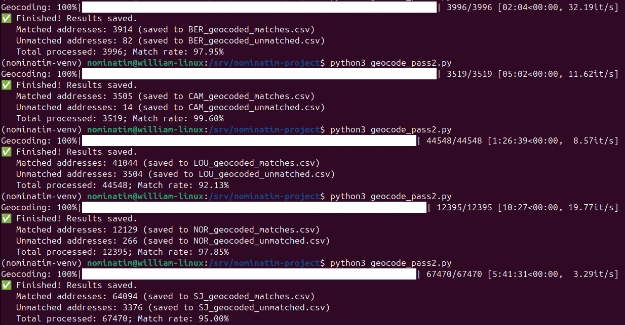
Results

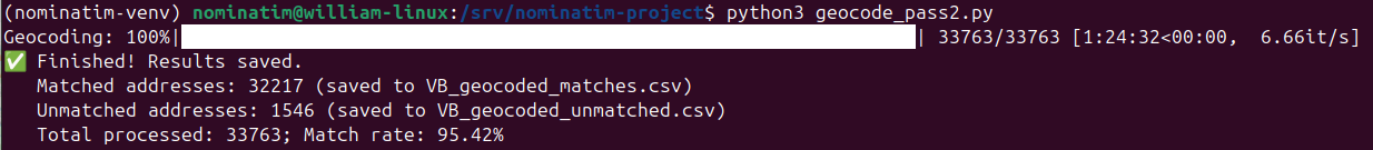
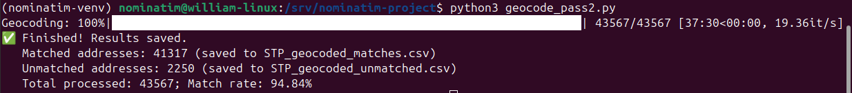
The result below is produced by running geocode_pass2.py (skipping geocode.py as geocode_pass2.py encompasses its functionality) on addresses from 7 actual crime datasets, each with its fair share of artifacts, but no parsing beyond those described above is done prior to geocoding. The exercise is carried out on a machine with an AMD Ryzen 5 9600X 6-core Processor, 96 GB RAM and 1 TB Gen 3 NVMe SSD; the PostgreSQL workflow implemented with ThreadPoolExecutor from concurrent.futures and connection pool from psycopg2 is very performant and will benefit fully from extra CPU cores (the CPU does run at 100% the entire time when paired with only a Gen 3 NVMe SSD), unlike R or Python programming where multithreading support is rather limited (the CPU may not run at 100% even with explicit implementation of multithreading). As discussed in previous parts, this project places heavy emphasis on accuracy, which is prioritized over match rate (and hence the strict enforcement of viewbox and cautious, convoluted fallbacks), nevertheless, with careful tuning and iterations based on unmatched addresses, it is possible to achieve results that rival those of some of the best commercial APIs , especially if there is not much flexibility for tuning or if trial and error get expensive.

The run time is dependent on both the number of addresses and the size of the viewbox which directly affects how many addresses have to be searched through in some of the steps because viewbox is essentially a filtering criteria. This is evident from the run time being much longer and number of iterations per second being much lower for larger cities, both in the sense of population (more cases and addresses) and area (more streets and intersections). Perhaps less obviously, the run time is also dependent on how well-formatted the addresses are, as each variant in Section 2.3 is tried sequentially and the code exits immediately upon the first match, this means an unmatched address will “drag on” for longer, this also means if some necessary fixes are put in place to cause an address to be matched earlier at say “2. abbr_expand” instead of unmatched, the code will actually run faster; in any case, the run time is still very manageable given that only an entry-level CPU is used.

Table 1: Geocoding results for 7 US cities, data from local police departments

Figure 4: Demonstration of geocoding results for Cambridge, MA

Copyright © April 2025. Hung Kit Chiu. Please do not circulate outside of UCSB Econ.